Converting a Text String to a Number in Calc

From NeoWiki

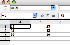
In a Calc document, sometimes it happens that some cells formatted in Text format contain Numbers, for example when the tables come from converted files, (such as converted .pdf files). In those cells, the numbers appear normally, but they are aligned to the left like strings of characters. If you click in a cell which contains such a number, for instance 23, you will see '23 in the formula bar. In order to convert those texts to numbers, you have a function available: the VALUE function.

Converting a text to a number

Let us assume that the cells A1, A2, A3 contain the texts 23, 12, 36. We are going to display the same values in the cells B1, B2, B3, but in number format.

• Click in the cell B1
• Click the minus sign "=" on the left side of the formula bar.
• type VALUE in the input line.
  • You can find that function by clicking the formula icon on the left side of the Σ sign. In the Function Wizard dialogue that opens, click the Functions tab, then the Text category and select VALUE.
  • Click Next.
• Click in the cell A1. Now it is bordered with a red rectangle.
• Press Enter or Return. The number 23 appears aligned to the right in the cell B1.
• Then select the three cells B1 to B3, by clicking the cell B1 then dragging the cursor to the cell B3, or by clicking the cell B1 then, pressing the Shift key, clicking the cell B3.
• Go to the Edit menu, then the Fill sub-menu and select Down.
  

The three cells B1, B2, B3 now contain the numbers 23, 12 and 36.

Removing the cells which contain texts

Now, you may want to delete the cells A1 to A3. Unfortunately, if you delete them the cells B1, B2 and B3 will contain only 0, since it is the value that the VALUE function assigns to an empty string.
In order to solve that ptoblem, you can simply hide the column A by right clicking (or Ctrl-click) the header of the column then selecting Hide.
Another method, more complex, allows you to really delete it.

1. Export the sheet in Texte CSV format:
   • In the File menu choose Save As….
   • In the Save window and in the File type drop down menu, choose Text CSV(.csv) and check Edit filter settings.
   • Click Save.
   • In the dialogue asking if you want to save the document in the .csv format, click Yes.
   • In the Export of text files dialogue, set the Field delimiter option to {Tab} .
   • Click OK.
2. Import the .csv file in a spreadsheet and remove the column A:
   • Open a Calc document (which can be the same as the one from which you exported a sheet in .csv format).
   • Go to the Insert menu and select the Sheet From File… sub-menu.
   • Choose the .csv file you created before.
   • In the Text Import dialogue, be sure that the Tab option is selected in the Separator options section.
   • Click OK.
     

A new sheet is added in which you can delete one of the two columns A or B. Now, both of them contain numbers.