Listing Unique Items in a Cell Range

From NeoWiki

Let us suppose you have a column in a spreadsheet whose several rows contain the same values. You want to be able to get a list of the unique items and to display the number of times each item appears in the first list. NeoOffice allows you to do that by using the VLOOKUP function.

Example
Let us suppose the range A1:A14 contains the names of the following colors, purple, red, blue, green, each of them appearing several times.
Apply the following method:

• Insert two new columns to the left of column A (the values of the column A have now moved to column C).
• Select the cell A1 and enter the formula

  =IF(COUNTIF(C$1:C1;C1)>1;0;1)

• Press the Return key.
• Copy this formula downwards (see Selecting and Filling a Cell Range).
• Select the cell B1 and enter the formula

  =SUM(A$1:A1)

• Press the Return key.
• Copy this formula downwards.

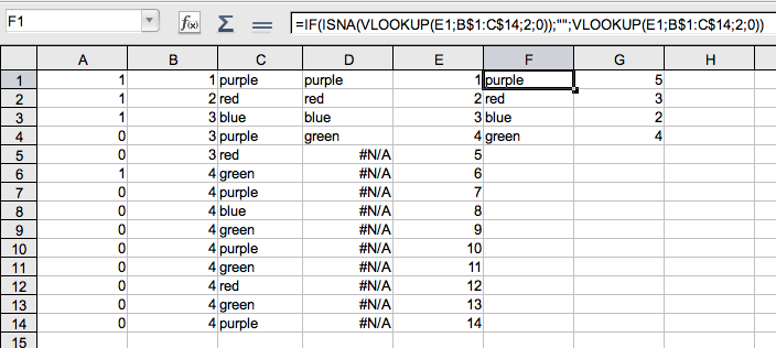
  You get a column containing the value 1 in front of the first occurrence of each color, and a column which contains the number of occurrences of each color.

• Create a range which contains the first 14 integers, e.g. E1:E14 filled with integers 1 to 14.
• Select the cell D1 and enter the formula

  =VLOOKUP(E1;B$1:C$14;2;0)

• Press the Return key.
• Copy this formula downwards.

  You will notice that as there are only 4 colors, starting from the fifth row you get the error message #N/A. Thus, we have to slightly modify the formula in order to fix that problem.

• Select the cell F1 and enter the formula

  =IF(ISNA(VLOOKUP(E1;B$1:C$14;2;0));"";VLOOKUP(E1;B$1:C$14;2;0))

• Press the Return key.
• Copy this formula downwards.
• Select the cell G1 and enter the formula

  =SUMPRODUCT(C$1:C$14=F1)

• Press the Return key.
• Copy this formula downwards.