Parsing Names in NeoOffice Calc

From NeoWiki

Revision as of 12:56, 18 August 2007 by Jgd (Talk | contribs)

(diff) ←Older revision | Current revision (diff) | Newer revision→ (diff)

Let us suppose that you have a column in a spreadsheet which contains names made up of several parts: first name, possibly middle name or initials, and surname. If you want to parse these names in order to get the three parts in three different columns, you can do it thanks to the functions included in NeoOffice Calc.
Proceed as follows:
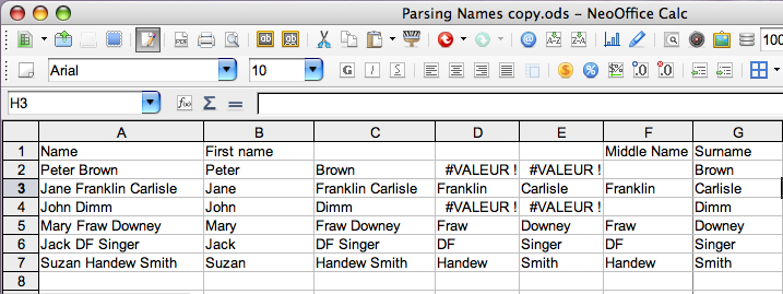
In this example, the full names are stored in the cell range A2:A7.

Displaying the first names in the range B2:B7

Select the cell B2, then enter in the formula bar the command:

=LEFT(A2;SEARCH(" ";A2)-1)

Press the Return key.
Click in the cell B2, and fill the range B2:B7 as described in this article.

The range B2:B7 contains now the first names.

Displaying the middle and first names

1) All the names are made of two parts, the first name and the surname.

Select the cell C2, then enter in the formula bar the command:

=RIGHT(A2;LEN(A2)-SEARCH(" ";A2))

Press the Return key.
Click in the cell C2, and fill the range C2:C7.

Those cells contain the surnames.

2) Some names are made of three parts, others of only two parts.

Then the situation is a bit more tricky, and you have to go through intermediary steps.

Select the cell C2, then enter in the formula bar the command:

=RIGHT(A2;LEN(A2)-SEARCH(" ";A2))

Press the Return key.
Click in the cell C2, and fill the range C2:C7.

The cells contain either the surnames or the middle names and the surnames together.

Select the cell D2, then enter in the formula bar the command:

=LEFT(C2;SEARCH(" ";C2)-1)

Press the Return key.
Click in the cell D2, and fill the range D2:D7.

Some cells display the error message "#VALUE!". They match the names which are made of only two parts. The other cells display the middle name (or initials).

Select the cell E2, then enter in the formula bar the command:

=RIGHT(C2;LEN(C2)-SEARCH(" ";C2))

Press the Return key.
Click in the cell E2, and fill the range E2:E7.

Again some cells display the error message "#VALUE!". They match the names which are made of only two parts. The other cells display the surname.

Select the cell F2, then enter in the formula bar the command:

=IF(ISERR(D2);"";D2)

Click in the cell F2, and fill the range F2:F7.

The cells of this range display the middle names, if any, otherwise they are empty.

Select the cell G2, then enter in the formula bar the command:

=IF(ISERR(E2);C2;E2)

Press the Return key.
Click in the cell G2, and fill the range G2:G7.

The cells of this range display the surnames.

Hiding/Showing the auxiliary columns

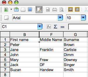
It remains to hide the columns C, D and F (and possibly the column A).

Select those four columns: click on the heading of the column A, then keeping pressed the Cmd key, click the headings of the columns C, D and E.
Go to the Format menu then to the Columns submenu and choose Hide.

If you add names in the column A, you will have to show those columns to parse those new names.

Select the sheet by clicking on the rectangle at the far left of the heading row, and go to the Format menu, then to the Columns submenu and choose Show.