|
|
Parsing Names in NeoOffice Calc
From NeoWiki
Let us suppose that you have a column in a spreadsheet which contains names made up of several parts: first name, possibly middle name or initials, and surname. If you want to parse these names in order to get the three parts in three different columns, you can do it thanks to the functions included in NeoOffice Calc.
Proceed as follows:
In this example, the full names are stored in the cell range A2:A7.
Displaying the first names in the range B2:B7
- Select the cell B2, then enter in the formula bar the command:
- =LEFT(A2;SEARCH(" ";A2)-1)
- Press the Return key.
- Click in the cell B2, and fill the range B2:B7 as described in this article.
The range B2:B7 contains now the first names.
Displaying the middle and first names
1) All the names are made of two parts, the first name and the surname.
- Select the cell C2, then enter in the formula bar the command:
- =RIGHT(A2;LEN(A2)-SEARCH(" ";A2))
- Press the Return key.
- Click in the cell C2, and fill the range C2:C7.
Those cells contain the surnames.
2) Some names are made of three parts, others of only two parts.
Then the situation is a bit more tricky. Using regular expressions and the SEARCH function is helpful.
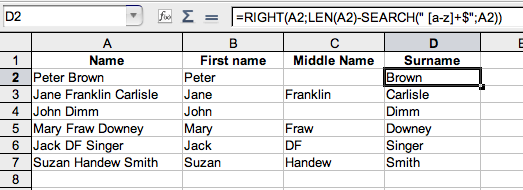
- Click on cell D2, then enter in the formula bar:
- =RIGHT(A2;LEN(A2)-SEARCH(" [a-z]+$";A2))
(Don't forget the quotes and the space before [a-z]+$).
- Press the Return key. You get the surname in D2.
- Fill the range D2:D7.
- Click on cell C2, then enter in the formula bar:
- =TRIM(MID(A2;SEARCH(" ";A2);LEN(A2)-LEN(B2)-LEN(D2)))
- Press the Return key.
- Fill the range C2:C7. The cells of this range display the middle names, if any, otherwise they are empty.
Hiding the column A
If you wish, you can hide the column A.
- Select this column by clicking on its heading .
- Go to the Format menu then to the Columns submenu and choose Hide.
If you add names in the column A, you will have to show that column to parse those new names.
- Select the sheet by clicking on the rectangle at the far left of the heading row, and go to the Format menu, then to the Columns submenu and choose Show.

